Locally adapted grayscale mapping
Locally adapted binarization
Global binarization
Grayscale image enhancement can be global or local, and examples of both are given here. Document images in particular can also be grayscale enhanced as a step either for grayscale image cleanup or as a precursor to image binarization.
However, image binarization is typically treated as simply a thresholding operation on a grayscale image, and we give standard global (Otsu) and local (Sauvola) thresholding operations in the following sections. In the following, we consider operations on document images, where text is foreground.
Several different implementations of adaptive mapping of grayscale images are given in adaptmap.c. The basic method is to determine the local background value and map the pixels linearly so that the background is put at some constant value like 150 or 200. There are two basic problems. The first is that there must be an actual local background. If there is an image on the page, it will be degraded if we try to force a background on it. So it may be important to do text-image segmentation first and then do background mapping only on the text parts. The second problem is to estimate the local background value. We do this efficiently by tiling the image, identifying pixels that are almost certainly not background, and finding the average of the non-background pixels in each tile. We require a minimum number of such pixels (typically about 1/3 of the pixels in the tile), and if there are fewer, we estimate the background value in the tile based on its neighbors. We additionally allow for smoothing between tile values, implemented by block convolution. Once the "image" of background values is established, the image can be mapped so the background is uniform across the full image. The image can then be binarized by selecting a global threshold that is somewhat below the background value.
A fancier adaptive mapping, pixBackgroundNormFlex(), is useful for situations where the background is changing very rapidly. It starts with image smoothing, using a scaling factor of about 1/5 or 1/7. This is a very cheap way to estimate the average pixel value in small tiles. A common problem is that there is thick text that is not very dark, and it is important not to treat the interior of such text as background. The approach taken is to use filling of grayscale basins to a height that is a given constant above the basin minima, and a local threshold can then be chosen to solidify the foreground regions without corrupting the background.
Another problematic situation is where the contrast between foreground and backgrond is very small, so that for binarzation it is important to choose the threshold carefully. We use a local contrast mapping, pixContrastNorm(), that computes and applies a local TRC (tone reproduction curve) to expand the local dynamic range to 8 bits, by mapping the darkest pixels to 0 and the lightest to 255. This is useful where the locally computed TRC function does not change rapidly with position.
Yet another approach is to compute a local threshold over the image and normalize the image so that the computed threshold is a constant. This approach is implemented with pixThresholdSpreadNorm(), which starts with a typically sparse set of estimates of the threshold value (determined by an edge detector). The estimated values are smoothed and then spread by a propagation method, giving a Voronoi-like result for regions with constant threshold value.
Binarization methods that use local adaptation are given in binarize.c.
The Sauvola method for local binarization does quite well, and we implement it with tiling for efficiency. The basic idea behind Sauvola is that if the is a lot of local contrast, the threshold should be chosen close to the mean value, whereas if there is very little contrast, the threshold should be chosen below the mean, by an amount proportional to the normalized local standard deviation.
Sauvola is implemented efficiently by using "integral image" accumulators for the mean and mean-squared pixel values. The latter requires 64 bit floating point arrays, which are expensive for large images. Consequently, we give a tiled version. This gives the identical results as the non-tiled method, but only requires accumulator arrays to be in memory for each tile separately.
The use of a local background normalization followed by a global threshold was discussed briefly above. Here we give a few more details. The local estimate of the background value in the grayscale image is used to linearly map the pixel values in such a way that the background goes to a global constant.
There are several parameters that must be selectdd for locally-adaptive background normalization:
Parameter selection depends on the expected spatial dependence of the local background. To track faster variation, it is necessar to use smaller tiles and a smaller smoothing convolution filter. However, using unnecessarily small tiles gives a noisier result.
Image binarization using a local background normalization, followed by a modified Otsu approach to get a global threshold that can be applied to the normalized image. The binarization is implemented by pixOtsuThreshOnBackgroundNorm().
Local background normalization of the grayscale image is done first, with the background being mapped to white (255). Then, to determine the threshold that should be applied, a modified Otsu threshold is found for the normalized image, and this is applied globally.
After local background normalization, two different thresholds are used. For the part of the image near the thicker text, a high threshold can be chosen, to render the text fully in black. For the rest of the image, much of which is background, use a threshold based on the Otsu global value for the original image. This binarization is implemented by pixMaskedThreshOnBackgroundNorm().
It is necessary to build a binary selection mask over the thicker or darker text, and use it to combine the two thresholded images. This selection mask is generated as follows. Do a second background normalization, this time with a very small tile size. The result is to create very light pixels in the background near significant edges. These pixels appear as a white halo around the thicker text, and they are extracted as a binary mask by high-pass thresholding. The mask is then solidified over the dark text by morphological dilation.
Then to extract the thick text, a high global threshold (say, 190) is used. The rest of the image is thresholded using a value derived from the modified Otsu method (described above) on the original image. Empirically, it is best to use a threshold value that is 30 greater than the Otsu value, in order to recover the lighter parts of the foreground.
Both thresholds can be applied to the standard normalized image where the background is mapped to 255, and the resulting 1 bpp images are combined using the selection mask.
There are many other possible variations for binarizing document images, using locally adaptive methods, but this should give you a feel for some of the approaches that can be used.
If an image has had its background normalized to a constant value, it can be binarized by a global value chosen to be less than the background by an appropriate amount. It must be less because the background cannot be made exactly constant, especially in situations where it was changing rapidly or where there is bleedthrough from text or image on the other side of the page.
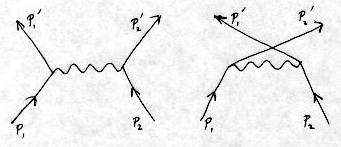
Alternatively, some images can be binarized well with a global threshold, and for these, one common approach is that due to Otsu. In standard Otsu, the different possible thresholds are used on the histogram of pixel values, and the threshold is chosen to maximize the variance of the two pixel distributions. Specifically, a score function is maximized that is the product of the number of pixels on each side of the threshold times the separation of the mean values. This works better when the ratio of the number of bg pixels to fg pixels is not too large. However, if there are few fg pixels, the threshold will be chosen well up the lower slope of the background distribution, resulting in many bg pixels being thresholded to fg. We use a modification of Otsu to moderate this effect. Instead of choosing the threshold value to be at the maximum of the score, we choose it to be at the minimum histogram value such that the score is within some fraction of the maximum.
We also give a somewhat locally adapted version of Otsu, by tiling the image (with the Pixtiling machinery) and determining the Otsu threshold separately in each tile. Again, there is an optional smoothing operation on the tile thresholds.
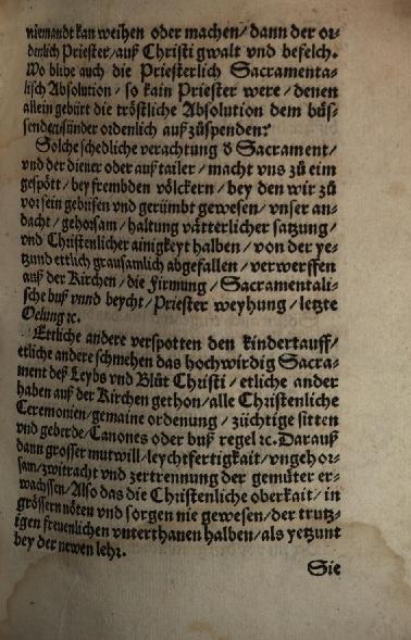
For clean images where there is not a large variation in the background pixels, or for images that have had their background normalized (as described above), Otsu works quite well. So why the modification? This is best shown by an example. Consider this image:
When we apply standard Otsu to this image (with scorefract = 0 in pixOtsuAdaptiveThreshold(), and using large numbers for sx and sy to guarantee a single tile over the entire image), we get a rather poor result:
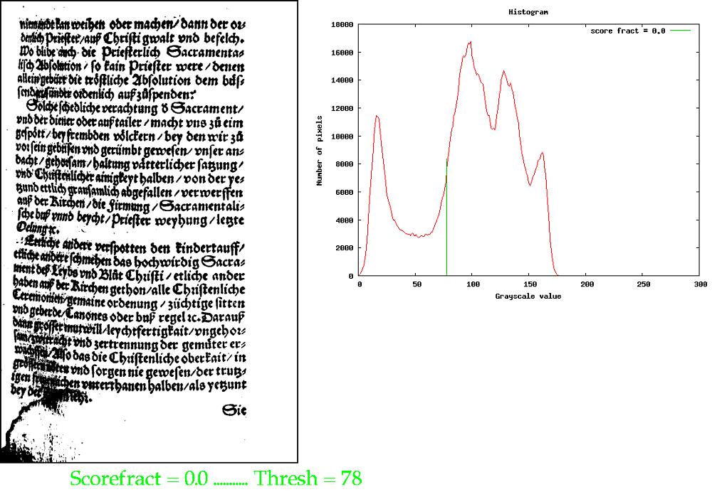
Some of the darker bg has been thresholded as fg. The origin of the problem is evident from the histogram, where the threshold sits up on the shoulder of the large background peak. However, by setting scorefract = 0.1, to allow the modified Otsu to choose the minimum in the histogram in a range where the score is within 0.9 of the maximum value, we get this:
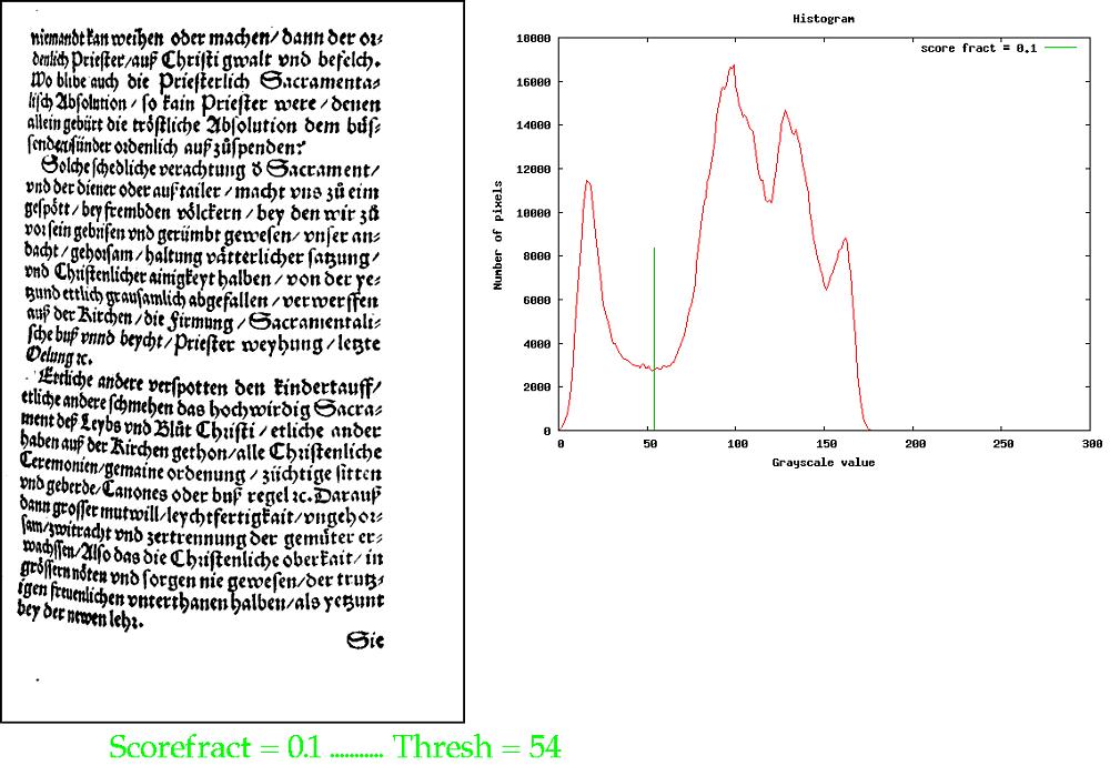
This is a significant improvement. However, notice that the text on the right side is relatively weak.
By tiling the image (adaptive Otsu) we can do a bit better. Choosing a tile size of 300 x 300, which must be considerably larger than can fit into the background at the bottom of the image, one obtains a much better result:
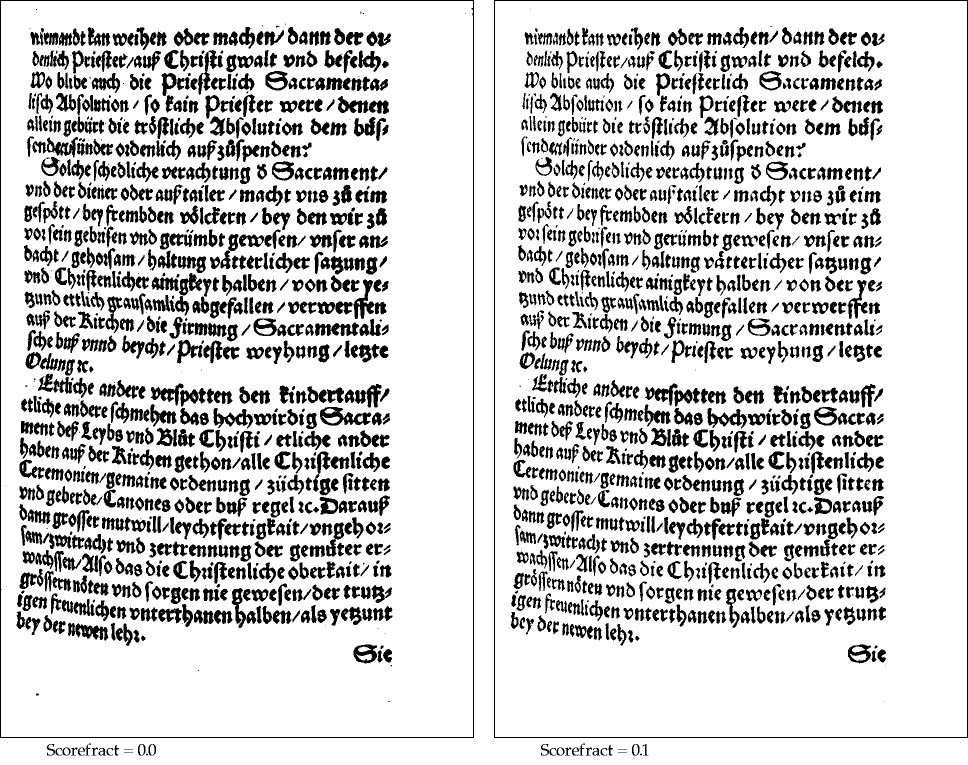
The result on the left is for standard (tiled) Otsu, with scorefract = 0.0, and on the right is modified (tiled) Otsu with scorefract 0.1. For both, most of the background is now properly assigned. On the left the text is a bit heavier throughout, and there is a small amount of noise in the background, but with modified Otsu the text is lighter and generally more evenly weighted.
That's about the best we can do with Otsu. When working with
difficult images, the various adaptive methods that do some
type of background normalization give better binarizations
than the global methods (of which Otsu is perhaps the best).
