1. What is a convolution?
2. Grayscale convolution
using an accumulator
3. Binary rank-order and median filter using an accumulator
Image convolution is a linear image processing operation where each dest pixel is computed based on a weighted sum of a set of (typically nearby) source pixels. For simplicity, label the pixels as a one-dimensional array. Let the n-th dest pixel have value bn, the p-th source pixel have value ap, and the digital filter F have a set of nonzero values Fm for some set {m}, where typically the filter Fm is normalized so that Sum{m}Fm = 1. The filter works as follows:
bn = Sum{m} Fm am - n (convolution)
for each dest pixel n. The sum over the m terms
in the convolution is the inner loop of the computation.
The order of the indices on the RHS is a convention
for the convolution, similar to the convention
for the indices in the morphological erosion. Reversing
the indices to take
cn = Sum{m} Fm an - m (correlation)
is called a correlation.
If the images are N x M pixels and the number of nonzero elements in the filter F is s, then the convolution requires NMs multiplications and additions. This grows linearly with the size of the convolution filter; for large filters and large images, the computation can be quite slow. However, one often needs to use a large filter. For example, a low-pass filter is used to remove high frequencies in the image, prior to subsampling. (See the discussion of anti-aliasing in the section on image scaling.) The lower the passband of the filter, the larger the required filter.
There is one special situation where the computation
does not depend on filter size; namely, where the filter
is rectangular and flat (i.e., with constant coefficients).
We describe here a method that convolves
an image with such rectangular flat filters of
arbitrary size, and that performs the
convolution in a time that is
independent of the size of the filter!
Essentially the same algorithm allows you to do fast median (and, more
generally, rank-order) filtering of
binary images.
What these methods both
have in common is the use of a pre-computed accumulator array.
A similar algorithm using a one-dimensional accumulator
of minimum or maximum values, rather than sums, can be used for fast
grayscale morphological filtering with flat one-dimensional filters.
Without the accumulator, grayscale morphological filtering
requires either a scan at each location to find the min or max,
or the maintenance of an ordered queue of pixel values as
pixels are added and removed.
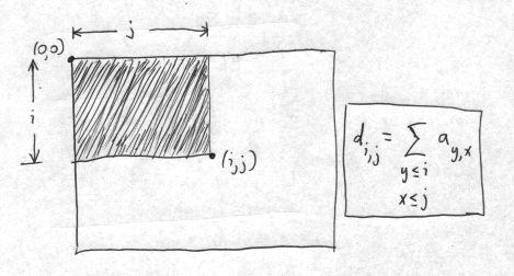
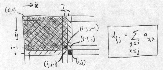
di,j = di,j-1 + di-1,j + ai,j - di-1,j-1 (accumulator)This recursion relation can be seen geometrically from the following diagram:
The convolution with a flat rectangular kernel of width w and height h is then found using the accumulator in the following way:
bi,j = [di,j + di-h,j-w - di,j-w - di-h,j] / wh (convolution using accumulator)This is the "inner loop" of the convolution, and it can be visualized as:
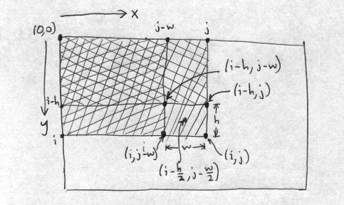
The equation for the convolution using the accumulator, as written above, has an unnecessary asymmetry in that the pixels used for the convolution are in the rectangle above and to the left of it. The average should instead be taken over pixels on all sides, so that the dest pixel is as close as possible to the center of the rectangle of source pixels used. We change parameters and let the full width and height of the convolution filter be 2w+1 and 2h+1, respectively. We can then write the convolution inner loop as
bi,j = [di+h,j+w + di-w-1,j-h-1 - di+h,j-h-1 - di-h-1,j+w] / (2w+1)(2h+1) (symmetric convolution using accumulator)With reference to the figure above, we are finding the dest pixel value in the center of the rectangle covered by the filter. In the figure this pixel was labelled by (i-h/2,j-w/2), but we are now labelling the dest pixel by (i,j). Note also that in the figure, the filter area is given as wh, not as (2w + 1)(2h + 1) in the above equation. In the equation, we still have a slight lack of symmetry in the convolution between the positive direction (e.g., i+h) and the negative direction (e.g., i-h-1). This is discussed in the source code in convolvelow.c.
We are not yet finished, because the boundary conditions must be handled properly. The accumulator is found recursively, looking up one row and left one column, so special cases need to be used for the top row and leftmost column of the array. Boundary effects on the convolution are more difficult. We have three choices: (1) ignore pixels where the convolution filter goes beyond the edge of the image, (2) do the best job you can with the pixels near the boundary, and (3) use mirrored pixels to compute near the boundary. For pixBlockconv(), we choose the second method. For pixels on the corners of the image, for example, we only have about 1/4 of the neighbors to use in the convolution that we have for pixels where the full filter can be used. The sum over those neighboring pixels should be normalized by the actual number of pixels used in the sum. The method we use is (1) for every pixel, use all possible pixels in the convolution, staying within the source image, but normalize as if we had used the entire filter, and (2) then make a second pass for the boundary pixels, adjusting the normalization upwards by the inverse of the fraction of the filter pixels that were actually used at each dest pixel. The first part gives values that are too small for convolutions near the boundary; the second pass increases these pixel values to their correct normalization, depending on exactly which row and column the pixel is in. Doing the normalization this way avoids overflow in the destination pixels. The result has no visible boundary pixel artifacts in the convolution for typical grayscale images.
An alternative approach, mentioned above, is to add mirrored border pixels, of sufficient size so that the accumulator array can be used at all points in the interior, corresponding to the original image, and without special-casing any pixels. This is implemented in pixBlockconvTiled(), where we also allow the convolution to be done independently in an arbitrary set of tiles of the image. The functions to generate the tiles and put the result back together after separate convolution, are found in pixtiling.c. If there is a single tile, the tiled convolution defaults to the original pixBlockconv. Otherwise, it is verified that the result of block tiling is identical to that given by the generic function pixConvolve(), for any tiling and kernel size. (Well, almost any: the constraint on the convolution size is that the convolution width must not exceed the tile width, and similiarly for the heights.)
Breaking the convolution up into tiles is useful in two situations.
First, if the grayscale image has more than 16M pixels, the accumulator
array, stored as a 32-bit unsigned integer, can overflow. For such
images, using tiles with less than 16M pixels is required. In addition,
because each tile is computed independently, the convolution can
be carried out in parallel, making use of multiple cores to provide
a linear speedup.
When applied to binary images, the rank-order filter takes a sum of pixel values followed by a threshold. It is asking if the number of ON pixels under the filter exceeds a given fraction of the total pixels under the filter. A median filter is a special case that gives an ON pixel if at least half of the pixels are ON. Median pixels are very useful for eliminating some types of noise. The rank-order filter is much less expensive on binary images because it is not necessary to order the pixels by value -- you just take a sum and apply a threshold. The rank threshold r is the fraction, between 0.0 and 1.0, of the pixels that are required to be ON.
Grayscale convolution with a flat filter also takes a sum, and we have seen that the accumulator allows you to take a sum over any rectangle of pixels very quickly. So the same accumulator can be used to apply a rank-order filter to binary images! For a rectangular filter of width w and height h, and using a rank r, the sum of ON pixels is thresholded by rwh.
We provide a bit more than this. The function pixBlocksum() takes a 1 bpp image and generates an 8 bpp image, using a rectangular convolution filter. It sums the ON pixels under the rectangular filter at each location, and normalizes to between 0 (all pixels OFF) and 255 (all pixels ON), taking into account the number of pixels under the filter at each location.
The rank-order filter uses this function. It first calls pixBlocksum() to compute the intermediate block sum image, and then thresholds it to generate the binary rank-order dest image.
For the high-level interface, we provide a function that
generates the accumulator image, and both the convolution
and rank-order functions can (re)use the accumulator. If
you are just running the convolution or rank-order filter once,
you can have the accumulator generated, used and destroyed
by using NULL as input for the accumulator.
