What is grayscale morphology?
Implementation using the van Herk/Gil-Werman algorithm
The Tophat and H-dome transforms
Generalization: rank order filters
If you are not familiar with binary morphology, you may want to read about it first.
As mentioned in the section on binary morphology, grayscale morphology is simply a generalization from 1 bpp (binary) images to images with multiple bits/pixel, where the Max and Min operations are used in place of the OR and AND operations, respectively, of binary morphology. The following should be noted:
For the general case of an arbitrary SE of size A, where A, the "area" of the SE, is the number of hits, the computation of the Max or Min requires A pixel comparisons on the src image for each pixel of the dest. However, things get more efficient when the SE is a brick, by which we mean it is a solid rectangle of hits. For a brick SE, dilation (or erosion) can be decomposed into a sequence of 2 dilations (or erosions) on 1-D horizontal and vertical SEs. Each 1-D grayscale morphological operation can be done with less comparisons than the "brute-force" method. Luc Vincent described one such method, that uses an ordered queue of pixels, given by the set of pixels currently under the SE. The queue is ordered so that the Min or Max can be read off from the end. When the SE is moved one position, one pixel is removed from the queue, and a new pixel is placed into it, in the proper location. Most of the work goes into sorting the queue to maintain the order.
More recently, van Herk, Gil and Werman have described an algorithm that uses a maximum of 3 comparisons for a linear SE, regardless of the size of the SE. This method is described below, and it is the method we have implemented here.
Some useful image transforms are composed of a sequence of grayscale
operations. For example, the tophat operator is often
used to find local maxima as seeds for some filling operation. It is defined
as the difference between an image and the opening of the
image by a structuring element of given size. Another
local maximum finder is called the h-dome operator, and
it uses a
grayscale reconstruction method for seed filling.
(Yes, with h-domes, you do a seed-filling operation to find
seeds for another operation!). These are discussed in detail
in the section
on tophats and h-domes below.
The van Herk/Gil-Werman (vHGW) algorithm is similar to our fast method for convolution with a flat kernel, where we first computed an accumulation matrix and then used it to quickly generate the convolution for any rectangular kernel. vHGW differs in that we compute a localized running Max (or Min) array that is specific to the size of the linear SE, and we then use the array to compute the result pixels locally (over a length equal to the SE size).
The vHGW algorithm was published by van Herk in "A fast algorithm for local minimum and maximum filters on rectangular and octagonal kernels", Patt. Recog. Letters, 13, pp. 517-521, 1992 and by Gil and Werman in "Computing 2-D min, median and max filters", IEEE Trans PAMI 15(5), pp. 504-507, 1993. (There appears to be some priority dispute, so I take a neutral position and give credit to both sets of authors.) This was the first grayscale morphology algorithm to compute dilation and erosion with complexity independent of the size of the SE. It is simple and elegant, and the surprise is that it was only discovered as recently as 1992. It works for SEs composed of horizontal and/or vertical linear elements, and requires not more than 3 pixel value comparisons for each output pixel. The algorithm has been recently refined by Gil and Kimmel, in "Efficient Dilation, Erosion, Opening and Closing Algorithms," given at ISMM (International Symposium on Mathematical Morphology) 2000, Palo Alto, CA, June 2000, and was published in Mathematical Morphology and its Applications to Image and Signal Processing, Kluwer Acad. Pub, pp. 301-310. They bring the number down below 1.5 comparisons per output pixel, at a cost of significantly increased complexity. Consequently, we'll describe and implement the original method.
We describe dilation; for erosion, substitute Min for Max. In brief, the image is divided into pixel groups of length L, where L, an odd number, is the size of the SE. We describe the case for a horizontal SE with its origin at the center position (L/2). Vertical SEs are handled similarly, except the pixels are selected in vertical groups. On each raster line of length w, we compute output pixels starting at x = L/2 (to avoid boundary effects) and operate on N = (w - 2 * (L/2))/L segments of length L. N takes this particular form to avoid boundary effects on the right side as well, so that the last segment of length L is guaranteed to have the SE entirely within the image at all L points. As a result, we do not evaluate the first L/2 pixels and, in the worst case, the last 3L/2 pixels. To get reasonable results on all pixels in the image, we embed the actual image in a larger image with these augmented dimensions, where the added border pixels are appropriately initialized (to 0 for dilation and to 255 for erosion). The algorithm proceeds for each group of L pixels in 2 steps. In the first, we form the running Max array; in the second, we evaluate the output pixel values.
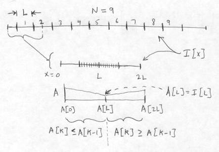
For each group of L pixels, we consider a window of 2L+1 pixels in the source image that extends L/2 pixels to either side. The pixel at the center of the L pixels is also at the center of this larger window. Form an array A[] of length 2L+1, consisting of backward and forward running Max pixel values, which are computed starting at the source pixel at the center of the group of L pixels. This array will coincide with the larger window of 2L+1 pixels. Now, consider the very first group in the raster. The larger window starts at the left edge (x = 0) and proceeds to x = 2L. The center value of the Max array, A[L], is given by the pixel at x = L. The value to the left of that, A[L-1], is given by the Max of the values of the pixel at x = L and the pixel at x = L-1, and so on progressively to the value at the beginning of the array, A[0], which is the Max of all pixels from x = L back to x = 0. The array values to the right of A[L] are likewise found by taking the Max of all pixels from x = L up to that point, progressing finally to the value at the end of the array, A[2L], which is the Max of all pixels from x = L to x = 2L. In all, this step requires computing 2(L-1) Max functions.
The generation of the running Max array A[] from the source image I is shown below. We display the domain over which a raster line of the image I is defined, but we do not display I[x] itself. As shown, there are N=9 pixel groups of length L for which output pixels can be computed. We magnify the first interval of length 2L+1 in I. This covers the relevant pixels in I that are used for generating the first pixel group of L output pixels in I':
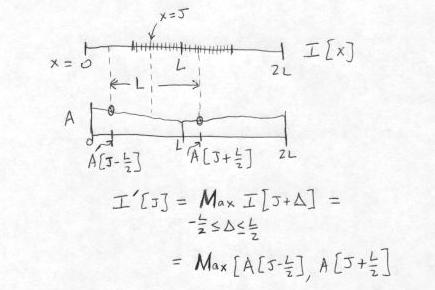
Once this array is formed, the values of the dilated pixels, that are written to the destination image, can easily be read off. For this first interval of length L, the L output image pixels from x = L/2 to x = 3L/2 are computed by imagining that the SE is placed on the array A with its center at one of these L locations; namely, at each pixel for which the SE fits entirely within the array A. We start at x = L/2, where the end points of the SE are at x = 0 and x = L, and take the Max(A[0], A[L]) = A[0]. (We know here that A[0] >= A[L], by the construction of the array A.) Then at x = L/2 + 1, we take Max(A[1], A[L+1]), and so on, up to the last value at x = 3L/2, which is Max(A[L] + A[2L]) = A[2L], again by construction. In all, this step requires computing L-2 Max functions.
The method for computing the destination (dilated) pixel values I'[J] from the source image I, for the first pixel group given by L/2 <= x <= 3L/2, is shown below. The computation of the output pixel at x = J is shown explicitly.
The total number of comparisons per output pixel is 3 - 4/L, which is never greater than 3. The calculation described above is repeated at each of the N segments of length L on the raster line.
The implementation is straightforward. We set up two buffers, one to hold an entire raster line (or column, for vertical SEs) of the image, and the second to hold the running Max(Min) array of size 2L+1. The raster line buffer is used to hold the pixels in byte order. For little-endian machines, this is exactly opposite to the standard pixel order for 32-bit words, which puts the pixels in MSB-to-LSB order; i.e., 3, 2, 1, 0. The pixel order in each 32-bit word is reversed as pixels are copied to the buffer. (For big-endian machines, no pixel reshuffling is necessary.) For vertical SEs, we just take the pixels in a column in order from top to bottom. See the source code in graymorphlow.c for other details.
As with binary morphology, opening and closing are defined
as a sequence of erosion/dilation and v.v. These operations
are idempotent, so one simple test for correctness is to
open an image with a SE and then open the result. The second
opening should give the same image as the original one.
Our implementation permits morphological operations with SEs that
are linear (horizontal or vertical) and square (implemented
as a sequence of horizontal and vertical operations).
The speed is independent of the size of the SE and proceeds
at about 120 P3 machine cycles per output pixel, for large images.
Binary segmentation most simply is carried out by selecting connected components in the image, using a seed image, a mask image (which is typically the actual image), and filling selected connected components in the mask that have seeds in them. Here, the mask is used to clip the filling process. In a more complicated situation, typified by a binary image of touching coffee beans, you need to split binary connected components. This can be done using the distance function and looking for low saddle points that are most easily cut through. How do you do that? Put the distance function upside-down. Then the seeds, which are the local maxima of the distance function (the points that are farthest from the boundaries) are at the bottom of the inverted function. The boundaries are at the highest point, and the "low passes" through the saddle are on the boundaries of the catchment basins. Segmentation is achieved by filling the basins to define the watersheds, which are all the points that drain into the same basin.
Similarly, grayscale segmentation usually proceeds by finding markers, or "seeds," and an image of catchment basins surrounded by walls at the boundaries. The catchment filling "mask" can be computed in various ways; a popular one is to use a properly smoothed morphological gradient, which has large peaks at places where the image intensity is rapidly varying -- a likely position to find a segmentation boundary. Filling then proceeds from the seeds into these basins.
There are various ways to get the seeds. Two popular ones are tophat and h-dome transforms. The tophat is simpler, and you can envision its operation as follows. Suppose you have a dark grayscale image with some small bright regions. To identify those regions, apply the tophat, using a SE that is larger than the extent of the regions. The opening is a Min operation that removes those bright regions that are smaller in dimension than the SE used in the opening. Then, subtracting this image with the thin peaks cut off from the original image gives you just those peaks, plus some low amplitude noise. The tophat is typically followed by a thresholding operation on the peaks. We've just described the white tophat. There is a black tophat that is a dual to the white tophat, and it subtracts the original image from the closing with a SE. The black tophat gives large pixel values in the result where there were small dark regions in the original image.
The h-domes are another method for finding local maxima. They use a grayscale reconstruction (seed filling) method, where the original image is the mask and the seed is derived from the mask by subtracting a constant value "h" from each pixel value. Reconstruction expands the seed into the original image (mask). This is visualized as having each local maximum of the seed expand horizontally until it hits a value of the mask that is of equal or greater value, at which point it can expand no further. To complete the h-dome transform, the filled seed is then subtracted from the original image, resulting in an image composed of the "domes" of local maxima of the original, none of which can exceed the value h in size.
You can find implementations of the tophat transform
pixTophat() and the hdome transform pixHDome() in
morphapp.c.
We have implemented both black and white tophat transforms,
even though they are trivially related. Intuitively, applying
a black tophat to find small dark regions should be equivalent to
applying a white tophat to the inverse of the image.
(The inverse of an image is found by replacing each pixel by its
reflection in the light-dark axis; specifically, if the pixel
has value v, it is replaced by the value 255 - v.)
And, in fact, this is correct. These operations have exactly
that simple duality relation:
the white tophat on an image is equal to the black tophat
on the inverse of the image, and v.v.
The proof, which uses the duality of the opening and closing
operations, is very simple.
Let the opening of an image I with a structuring element S
be given by OS(I), and the closing of I by S be
CS(I). From here on, due to a typographic
limitation of HTML, we'll suppress the "S".
Denote the inverse of an image I by I, where I = 255 - I.
The opening and closing are dual, in the sense that
O(I) = C(I). (Note that this is a different
sense of "dual" than for the black and white tophats, which we
are in the process of showing.) Denote the white tophat by
Tw(I) = I - O(I) and the black tophat by Tb(I) = C(I) - I.
Then the black tophat on the inverse of I is given by
Tb(I) = C(I) - I = O(I) - I =
255 - O(I) - 255 + I = I - O(I) = Tw(I)
which is the result that was to be proven. By the way, the
duality relations for opening and closing,
O(I) = C(I), or C(I) = O(I),
can be stated in words in several ways.
Here's one for the second of the pair:
The closing of an image can be equivalently
found by inverting the opening of the inverted image.
This holds for binary as well as grayscale, of course.
High frequency noise, which is not well filtered by the white tophat, can be greatly reduced by doing a closing first. Likewise, an opening is often necessary before a black tophat. The size of the SE in the opening or closing can be comparable to that used in the tophat.
(Parenthetical note. For seeing the results
clearly, we provide a function pixMaxDynamicRange()
that expands the dynamic range to cover the full set of 256
values for an 8 bpp image. We let you do this with either
a linear or log transform. The latter is useful for images
that cover a large dynamic range to begin with and have small
values that you wish to see and which appear black on a linear
scale.)
The brute force method is to sort all the neighboring pixels, and pick the value of the r^th one. The best sorting algorithms are O(n*logn), where n, the area of the filter, is the number of values to be sorted. For a 50x50 filter, the number of operations at each pixel is over 10,000, which is not practical. (These are not machine operations.)
However, we only need the r-th largest pixel. So our problem is really a "selection" one (e.g., quickselect), not a sorting problem. Now it turns out that using a variation of quicksort, selection of any specific rank value is O(n). This is because for selection you only need to sort the appropriate segment at each bifurcation in the quicksort method, rather than the entire tree. (For details, see Numerical Recipes in C, 2nd edition, 1992, p. 355ff.) There is a constant 2 in front of the n, relative to quicksort, so this brings the count down to 5,000 for our example, which is still ridiculously large.
Actually, we only need to do an incremental selection or sorting, because moving the filter down by one pixel causes one filter-width of pixels to be added and another to be removed. Can we do this incrementally in an efficient manner? Perhaps, but I don't know how. The sorted values will be in an array. Even if the filter width is 1, we can expect to have to move O(n) pixels, because insertion and deletion can happen anywhere in the array. By comparison, heapsort is excellent for incremental sorting, where the cost for insertion or deletion is O(logn), because the array itself doesn't need to be sorted into strictly increasing order. The heap, which is represented by an array, only needs to be in "heap" order, so just a few elements must be rearranged. However, heapsort only gives the max (or min) value, not the general rank value.
The conclusion is that sorting and selection are far too slow. All is not lost, because we can still use a histogram of pixel values. But how is this to be represented?
Suppose we represent the histogram as an array of 256 bins, which is the usual situation. At each new filter location, the histogram must be updated and the rank value computed. The problem we face is that, in general, to find the rank value, a significant fraction of the entire histogram must be summed. Suppose the filter size is 5x5. There are at most 25 different bins occupied, and we will mostly be adding zeros to the sum of bin occupancies. That is painful!
We can instead use a linked list, so that there won't be any unoccupied cells and the sum can be quickly done. However, we lose random access for insertion and deletion, so those operations become unacceptably slow.
However, we can mostly overcome the empty bin problem and retain random access by using two histograms represented as arrays, with bin sizes 1 and 16. Each of these histograms is updated for each pixel added or removed when the filter is moved. To find the rank value, proceed from coarse to fine, first locating the coarse bin for the given rank value, of which there are only 16. Then for the fine histogram with bin size 1 and 256 entries, we need look only at a maximum of 16 bins. On average, there will be a total of about 16 sums.
